Simulating the impact of layer exchange on temperature programmed desorption

The desorption of molecules or atoms from surfaces is pivotal for a large variety of natural and technological processes such as dewetting and catalysis. Hence, desorption processes has been studied intensively in the past. A powerful method to do so is temperature programmed desorption (TPD) as it can be used to gain mechanistic insights into the kinetics of desorption. To this end, it is a common procedure to analyse TPD data with analysis methods based on the Polanyi-Wigner equation as those methods can yield information on the order, energy barrier and entropy change of a desorption process. However, the Polanyi-Wigner equation assumes a single desorption path, which might lead to problems for real systems with multiple coupled desorption paths. For example, even if single-crystal surfaces are considered, an exchange between various adsorption positions such as step edges, kink sites, defects and adsorption sites in the second adsorbate layer is possible.

Two-layer model

To elucidate the influence of exchange between the first and second adsorbate layer on the kinetics of desorption we developed a kinetic rate model, which describes a two-layer system in terms of a model geometry and the relevant elementary processes. As part of this model, molecules (or atoms) referred to as particles adsorb in a regular array on a support surface. We investigate two layers of particles on the surface, where the particles can either adsorb directly on the surface (first layer) or on top of other particles (second layer). Particles can only reside in the second layer if all adsorption sites underneath are occupied as we assume particles on top of unoccupied adsorption sites to be in an intermediate state rather than at a stable adsorption site. Moreover, we consider a system without lateral interactions between particles.

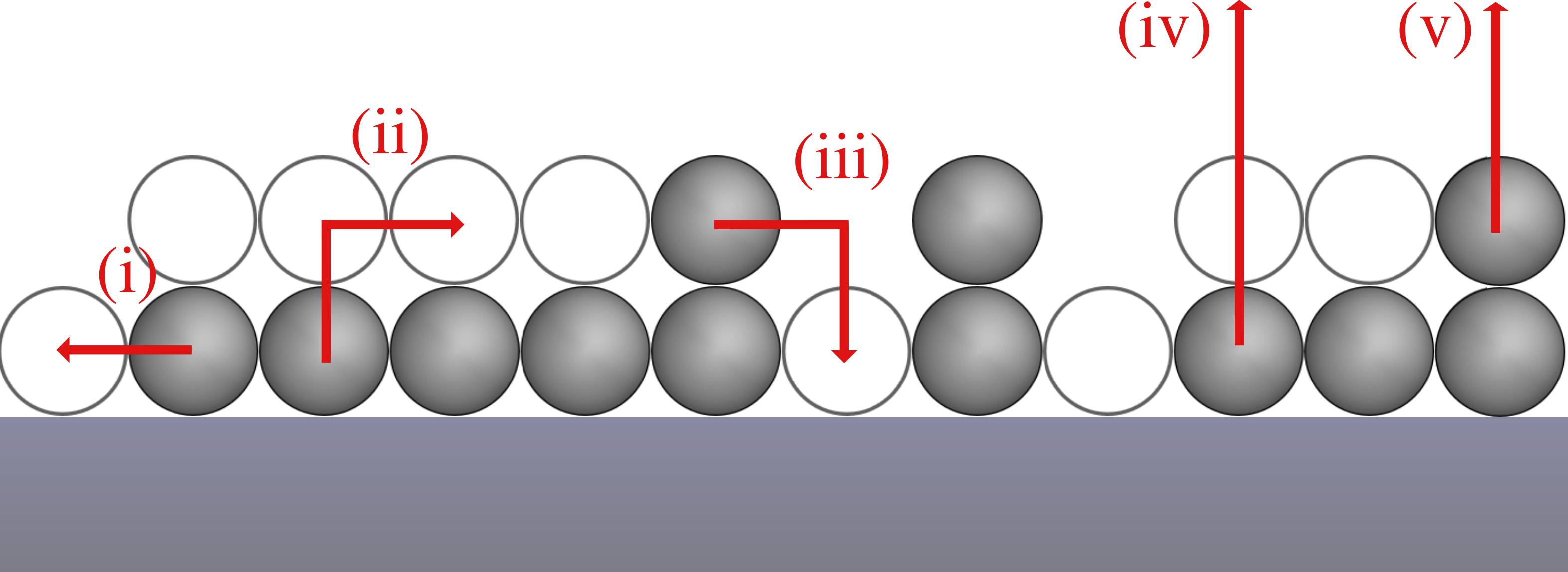
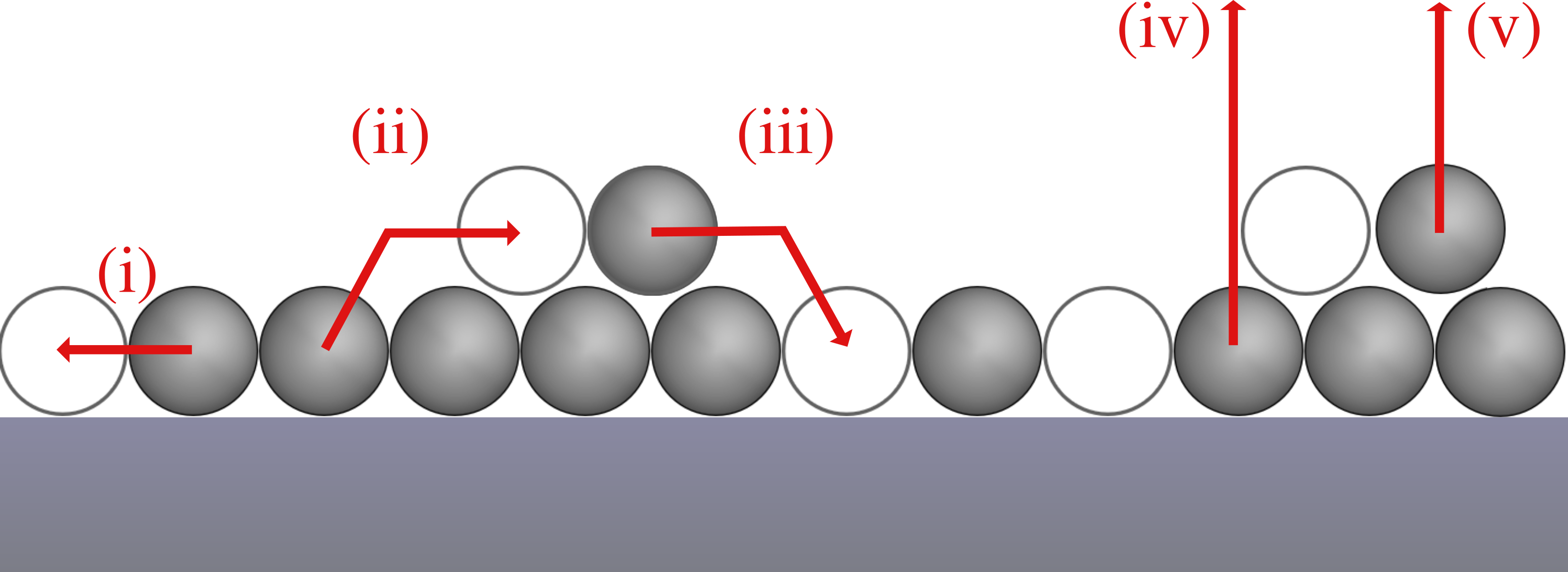
In terms of processes, our model includes the following elementary steps (see Fig. 1):

Diffusion: Diffusion (i) of particles within their layer is only treated implicitly by the assumption that the in-layer-diffusion is always in equillibrium. Thus, the particles are distributed randomly on the surface as we also consider a system without lateral interactions.
Layer exchange: Particles can change from the first to the second layer (ii) and from the second to the first layer (iii) if there is a vacant adjacent adsorption site in the other layer. Additionally, layer exchange from the first to the second layer requires that the particle in the first layer is not blocked by particles on top.
Desorption: We consider desorption from the first (iv) and second (v) layer, but with different desorption kinetics. Particles in the first layer can only desorb if there is no particle on top of them and are otherwise blocked. Particles in the second layer can always desorb.

The model geometry determines how the particles are arranged on the surface relative to each other. In principle, our model can be applied to various geometries. For the present visualisation, however, we provide a selection of possible adsorption geometries to chose from (see drop down list below). The current geometry is displayed in Fig. 1 and explained in the text below the drop down list.

Model geometry:

A one-dimensional chain of particles where the particles in the second layer reside directly on top of the particles in the first layer (same x coordinate, but different z coordinate).

Show differential equations

**Fig. 1** Schematic representation of the model geometry and elementary processes. The displayed processes are diffusion (i), layer exchange from the first to the second (ii) and from the second two the first layer (iii) as well as desorption from the first (iv) and second (v) layer. Occupied adsorption sites are displayed as filled spheres, while unoccupied adsorption sites are shown as empty spheres.

Gibbs free energy landscape

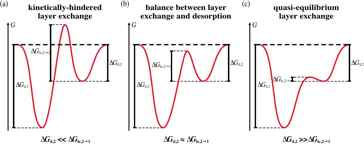
To elucidate the influence of layer exchange on the desorption process, we consider three cases for our model. Namely, we investigate (a) kinetically-hindered layer exchange, (b) balance between layer exchange and desorption and (c) quasi-equilibrium layer exchange. In case (a), kinetically-hindered layer exchange, layer exchange is considerably slower than desorption, thus, layer exchange does not take place on the timescale of desorption. This corresponds to a significantly higher energy barrier for layer exchange than for desorption as presented in Fig. 2 (a). In case (b) the rates of layer exchange and desorption are on the same order in both layers, which is why the kinetics of desorption are governed by a balance between layer exchange and desorption. In terms of free energy this means that $\Delta G_{\text{d,2}}\approx\Delta G_{\text{le},2\rightarrow 1}$ (see Fig. 2 (b)). Case (c) is characterised by significantly faster layer exchange than desorption, i.e., a significantly higher energy barrier for desorption than layer exchange (see Fig. 2 (c)). Hence, layer exchange is in a state of quasi-equilibrium on the timescale of desorption.

Fig. 3 shows a schematic free energy landscape calculated from the kinetic parameters specified in the grey box below, where we provide one example for each case as a starting point. The sliders can be used for a custom change of the parameters. The free energy landscape, in turn, can be compared to the case scenarios shown in Fig. 2 to see which case is applicable to a specific set of parameters. Please note that there are mixed cases as well, where the case changes in the relevant temperature interval.

In the next section, the parameters specified here can be used for the calculation of desorption spectra.

Parameter set:

Show in-depth discussion on cases and their stability?

**Fig. 2** Schematic Gibbs free energy diagrams for the three cases discussed here, which are kinetically-hindered layer-exchange (a), balance between layer exchange and desorption (b) and quasi-equilibrium layer exchange (c). In this scheme the free energy landscape is characterised by the barriers for desorption from the first and second layer $\Delta G_{\text{d,1}}$ and $\Delta G_{\text{d,2}}$ , respectively, and the barrier for layer exchange from the second to the first layer $\Delta G_{\text{le},2\rightarrow 1}$ .

Fig. 3 Schematic free energy landscape for the simulated model system at the temperature specified with the slider below.

In Fig. 2, we considered rather extreme examples, which clearly correspond to one of the three cases. For sets of kinetic parameters in the intermediate range between two cases, however, an intuitive classification might fail. Therefore, we discuss in detail how different kinetic parameters correspond to the three cases discussed above. To this end, we determine which conditions are necessary for the rates of layer exchange and desorption to be equal in the first and second layer and how to express these conditions in terms of the energy barriers of the system.

First layer: In the first layer, we compare the rate of layer exchange from the first to the second layer with the first-layer desorption rate. Those rates are identical if:

$2k_{\text{le},1\rightarrow 2} (\theta_1-\theta_2)^2=k_{\text{d,1}}\theta_1$

When we use the expression for the rate constants in terms of transition state theory and $\Delta G_x=\Delta E_x-T\Delta S_x$ , the equation above can be rearranged to:

$\Delta G_{\text{le,}2\rightarrow 1}-\Delta G_{\text{d,2}}=k_B T \ln\left(2(\theta_1-\theta_2)\right)$

Second layer: When we apply the same derivation as shown for the first layer we obtain for the second layer

$2k_{\text{le},2\rightarrow 1} (1-\theta_1)\theta_2=k_{\text{d,2}}\theta_2$

and

$\Delta G_{\text{le,}2\rightarrow 1}-\Delta G_{\text{d,2}}=k_B T \ln\left(2(1-\theta_1)\right)$

We can use these equal-rate-equations for the first and second layer in order to determine which case applies for a given set of kinetic parameters and temperature. To this end, Fig. 4 shows $\frac{\Delta G_{\text{le,}2\rightarrow 1}-\Delta G_{\text{d,2}}}{k_BT}$ as a function of the first- and second-layer coverages, where the surface of equal rates in the first (second) layer is displayed in red (blue). For the specific kinetic parameter set specified in the last section the same quantity ( $\frac{\Delta G_{\text{le,}2\rightarrow 1}-\Delta G_{\text{d,2}}}{k_BT}$ ) can be calculated and is displayed in Fig. 4 as a black plane. This means that the rates of desorption and layer exchange are equal at the intersection of the black plane with an equal-rate surface. Moreover, desorption is faster (slower) than layer exchange in one layer if the black plane is above (below) the corresponding equal-rate surface. The difference between the black plane and the equal rate surface is a measure for the difference in rates. Hence, Fig. 4 shows which case applies for a given set of kinetic parameters by evaluation of the difference between the equal-rate surfaces and $\frac{\Delta G_{\text{le,}2\rightarrow 1}-\Delta G_{\text{d,2}}}{k_BT}$ along the path of a desorption spectrum in terms of $T$ , $\theta_1$ and $\theta_2$ . However, the evaluation of Fig. 4 along the path of a desorption spectrum requires the knowledge of this path and, thus, of the desorption spectrum. As this information is not available beforehand, we provide a simplified case stability diagram (Fig. 5) for practical purposes.

For the simplified case stability diagram we used Fig. 4 to find critical values for the change between the cases. To ensure case (a) (case (c)) the term $\frac{\Delta G_{\text{le,}2\rightarrow 1}-\Delta G_{\text{d,2}}}{k_BT}$ has to be larger (smaller) than 6 (-8). In the intermediate range a case (b) applies. These critical values are independent of the first- and second-layer coverages, so the only remaining variable for the desorption path is the temperature. As a consequence, we can determine the case from a plot of $\frac{\Delta G_{\text{le,}2\rightarrow 1}-\Delta G_{\text{d,2}}}{k_BT}$ as a function of temperature as shown in Fig. 5. If $\frac{\Delta G_{\text{le,}2\rightarrow 1}-\Delta G_{\text{d,2}}}{k_BT}$ is smaller than -8 case (c) is applicable (cyan area). Between -8 and 6 the desorption spectrum is governed by case (b) and for values of $\frac{\Delta G_{\text{le,}2\rightarrow 1}-\Delta G_{\text{d,2}}}{k_BT}$ greater than 6 we can apply case (a) (violet area).

If the case changes in the course of a TPD experiment (black curve changes region) it needs to be considered that equilibrium condition is displayed in Fig. 5 which is not necessarily reached in the experiment.

Fig. 4 Difference

\frac{\Delta G_{\text{le,}2\rightarrow 1}-\Delta G_{\text{d,2}}}{k_BT}

as a function of the first- and second-layer coverages (move the 3D graph with the mouse to see

\theta_2

). The equal-rate surfaces for the first and second layer are displayed in red and blue, respectively, and the

\frac{\Delta G_{\text{le,}2\rightarrow 1}-\Delta G_{\text{d,2}}}{k_BT}

value calculated from the specified kinetic parameters and temperature is shown as a black plane. Hence, the rates of layer exchange and desorption of the current system are equal at the intersection between the black plane and the equal-rate surfaces. If the black plane is above (below) an equal-rate surface the desorption rate is higher (smaller) than the rate of layer exchange in the corresponding layer.

Fig. 5 Simplified case stability diagram. The Gibbs free energy difference

\frac{\Delta G_{\text{le,}2\rightarrow 1}-\Delta G_{\text{d,2}}}{k_BT}

is displayed as a function of temperature for the specified kinetic parameters. Those parts of the diagram, where layer exchange is kinetically-hindered (case (a)), are displayed in violet and those parts, where layer exchange is in equilibrium (case (c)), in cyan. For the assignment of these classification areas critical

\frac{\Delta G_{\text{le,}2\rightarrow 1}-\Delta G_{\text{d,2}}}{k_BT}

values were used as explained in the text. Moreover, the start and end temperatures of the TPD experiment (i.e. the relevant temperature range) are marked with ticks on the temperature axis.

Desorption spectra

The desorption spectra in the figures on the right-hand side are calculated numerically based on our two-layer-model and the kinetic parameters specified above. For the calculation we provide two algorithms. One algorithm integrates the model differential equations with a 4th order Runge-Kutta algorithm with variable timesteps. We refer to this algorithm as "full simulation". The other algorithm calculates desorption spectra under the assumption of an equilibrium state for layer exchange. In order to do so this algorithm uses a 4th order Runge-Kutta algorithm combined with a Newton-Raphson algorithm to find the equilibrium coverage distribution for layer exchange.

We use the "full simulation" algorithm for systems where the rates of layer exchange and desorption are comparable or desorption is faster than layer exchange. In contrast, we use the "layer exchange equilibrium" algorithm when layer exchange is significantly faster than desorption. This procedure is necessary, because a fast layer exchange requires our calculation to take (very) small timesteps on the timescale of desorption, which increases the computing effort significantly. While this might not be a problem for powerful computers this visualisation is intended to work on average personal computers as well. Hence, we need to keep the computation effort low. Moreover and more importantly, the "layer exchange equilibrium" algorithm provides excellent results if the energy barrier for layer exchange is indeed sufficiently low for case (c) to apply.

As a consequence, the "full simulation" algorithm only works for cases (a) and (b) (as the minimum timestep is restricted) and the "equilibrium layer exchange" works for case (c).

Technical notes: The calculation of desorption spectra with the "full simulation" algorithm can take several seconds to minutes depending on your system (e.g. 60s/spectrum on a 2,2 GHz 6-Core Intel Core i7 with 16 GB DDR4 RAM). Moreover, this visualisation was developed for Google Chrome, which is why we recommend viewing our visualisation with Google Chrome.

Simulation parameters

simulation mode

simulated data

dosing

advanced settings

show previous?

Fig. 6 Simulated desorption spectrum (a) and total coverage as a function temperature (b) for a two-layer system according to our model (violet). The contributions of desorption from the first (red) and second (blue) layer are shown in (a) and the corresponding coverages in (b).